-
[TAF] 시계열 Air Passenger Forcasting Project전공&대외활동 이야기/전공 프로젝트 모음 2024. 7. 1. 16:34
과제
uploaded dataset(AirPassengers.csv) provides number of monthly passengers of airlines over a period of 12 years (from 1949.01 to 1960.12). Please find the best ARMA model by satisfying the conditions in below.
- Use the first 10 years for estimation and rest of 2 years for one-step ahead forecasting.
- Please check the stationarity. If needed, you may need to use a d-th difference of yt or ARIMA(p, d, q).
- Based on ACF and PACF, suggest at least three candidate models with appropriate description.
- Evaluate the best model in terms of estimation (best fit) and forecasting performance.
- [ Extra 5 Points for Total Score in Class ] Add seasonality into the ARIMA model (Seasonal ARIMA).
정리하면 시계열의 정상성을 확인하고, 가능한 경우 ARIMA를 사용하고 가능한 경우 SARIMA를 추가하는 과제이다.
Dataset
우선 dataset은 Airppassenger데이터로 1949.01 to 1960.12까지의 월별 승객수를 기록한 것이다. 데이터 중 일부는 아래와 같다.

data 예시 연도와 월이 적힌 timestampl data와 승객의 수가 적힌 두 열로 구성되어있다. 이후 전체 dataset을 문제에서 정의한 것과 같이 In-sample data와 out sample data로 분리한다.
# genrally in time series we use in-sample and out-sample as a term but I prefer train, test for code
train = data[:'1958-12-01']
test = data['1959-01-01':]
In-sample 데이터를 기반으로 정상성을 확인하고 모델의 인자를 설정하며, Out-sample은 prediction 성능을 확인하는데에만 사용하도록 하자.
Check Stationary(Insample data)
우선 정상성을 확인하기 위해 원데이터, 1차 차분 data, 2차 차분 data를 생성한다. pandas에서 제공하는 diff를 통해 쉽게 차분이 가능하다.
이후 이를 시각화 하여 그림을 확인하자.
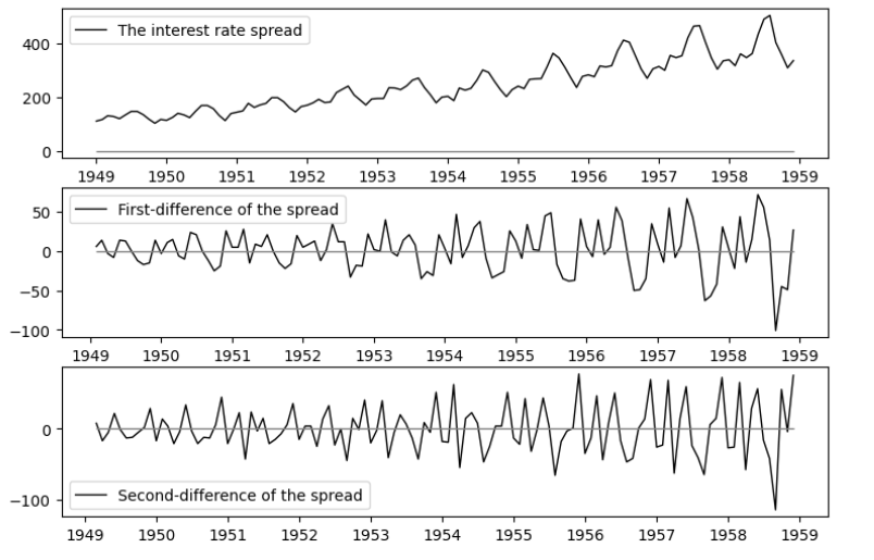
Fig 1: plot of the number of passenger, first difference, second difference 그림을 보면 증가하는 트랜드가 존재하는 것 처럼 보이며, sturctual break는 보이지 않아 보인다. 그럼으로 원데이터는 non-stationary하다고 시각적으로 결론 지을 수 있다. 또한 1차 차분과 2차 차분에서도 volatitliy가 증가하는 추세인것처럼 보이기 때문에 별도의 변형이 필요할 것으로 결론지었다. 필자는 log변환을 이용하였다.
log변환을 각각의 데이터에 적용할 경우 아래와 같다.

Fig 2: Plot of log transformed data and differences for log transformed data 보면 log 변환 전에 비해 꽤나 정상성을 띄는 데이터의 모습을 하고 있음을 확인 가능하다.
이후 ADF와 KPSS test를 통해 다시 이를 확인해보았다.
ADF&KPSS test: Stationary test
정상성은 Time series에서 매우 주요한 특성 중 하나로 아래의 ADF와 KPSS test에 의해 검정 가능하다.
ADF test의 경우 귀무가설(H0)로 unit root가 존재한다를 가지며 기각될 경우 정상성을 가지는 데이터라고 판단 가능하다.
Data type Statistics p-value Origin data -0.7734607708969381 0.8267937485032447 First differenced data -2.1641431278047762 0.21951577637150677 Second differenced data -13.947363642065772 4.7704196840302815e-26 First differenced
log-transformed data0.15822839568723085 0.15822839568723085 Second differenced
log-transformed data-7.633351316530781 1.981881694590538e-11 KPSS test의 경우 귀무가설(H0)로 Stationary data이다를 가짐으로 기각되지 않을 경우 정상성을 지니는 데이터라고 할 수 있다.
Data type Statistics p-value Origin data 1.7058124992217791 0.01 First differenced data 0.019023125650029386 0.1 Second differenced data 0.08275298336937394 0.1 First differenced
log-transformed data0.029471641004343525 0.1 Second differenced
log-transformed data0.409180392862506 0.1 결과를 통해 2차 차분한 데이터에서 모두 정상성을 지님을 확인 가능하다(1차차분의 경우 ADF는 통과하지 못하지만, KPSS는 통과하나 것을 확인 가능하다, 이 경우 대다수는 KPSS를 더 신뢰하나 본 프로젝트에서는 보다 보수적으로 접근하였다)
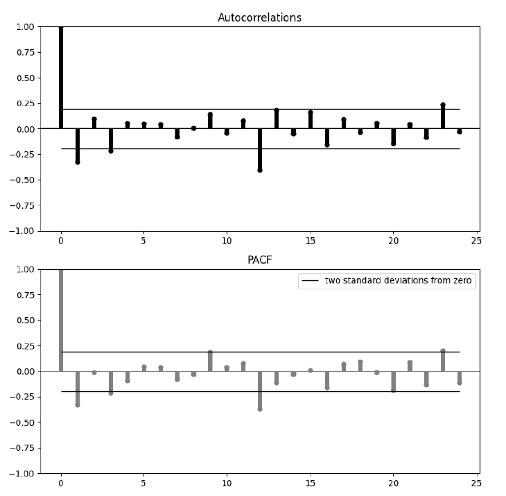
ACF & PACF make candiate
ACF와 PACF를 통해 ARMA(p,q)와 ARIMA(p,d,q)의 p와 q를 결정할 수 있다. 자세한 설명은 생략한다, 아래의 표를 보자.

ACF, PACF해석 d=1인 경우

1. The ACF and PACF show us a cyclical(seasonal) pattern(12), which seems like they has seasonality
2. The ACF does not cut to zero so that we can rule out a pure MA(q) process.
3. The ACF plot shows significant spikes at lag 1, 12, and 24.
There is a gradual decay in the autocorrelations. These patterns suggest the presence of seasonal components, given the regular spikes at higher lags.
4. PACF analysis
The PACF plot shows significant spikes at lag 1, 8, 10, 12. The initial spike at lag 1 indicates that an AR(1) component may be necessary. The PACF does not cut off quickly, which could indicate a mixture of autoregressive components and/or seasonal autoregressive components.
So for the given information suggested model are
1. since the series has been difference, d=1
2. significant spike at lag 1 in PACF suggests AR(1). p=1
3. significant spike at lag 1 in ACF suggests MA(1). so q=1 or 0, [1,4]
d=2인 경우

1. The ACF and PACF show us a cyclical pattern(12), which seems like they has seasonality
2. The ACF does not cut to zero so that we can rule out a pure MA(q) process.
3. ACF
The ACF plot shows significant spikes at lag 1 and 12, with the spikes decaying slowly over time. This suggests the presence of a seasonal component around lag 12. The spike at lag 24 is also notable and might suggest another seasonal cycle, but the primary focus should remain on the first noticeable seasonality at lag 12.
4. PACF
The PACF plot shows a significant spike at lag 1 and 2, indicating a possible AR(1) or AR(2) component. The significant spikes at lags 10,11,12 seasonal autoregressive components at these lags.
So for the given information suggested model are
1. since the series has been difference, d=2
2. significant spike at lag 1 in PACF suggests AR(1), AR(2). p=1, 2
3. significant spike at lag 1,2 in ACF suggests MA(1), MA(2). q= 0, 1, 2(I just test q=0 for sure)
d=1, log-transformed인 경우

1. The ACF and PACF show us a cyclical pattern (12), which seems like they have seasonality
2. The ACF does not cut to zero so that we can rule out a pure MA(q) process.
3. ACF: Significant spikes at lags 1, 12, and 24.
4. PACF: Significant spikes at lag 1 and 4 also at 10~12
So for the given information suggested model are
1. since the series has been difference, d=1
2. significant spike at lag 1 in PACF suggests AR(1), AR([1,4])
3. significant spike at lag 1 ACF suggests MA(1), MA([1,4])
d=2, log-transformed (ACF, PACF)

ACF and PACF show us a cyclical pattern(12), which seems like they has seasonality
2. The ACF does not cut to zero so that we can rule out a pure MA(q) process.
3. ACF: Significant spike at 1,4 / 12
4. PACF: Significant spike at 1,2,4 and 10,11,12
So for the given information suggested model are </br>
1. since the series has been difference, d=2
2. significant spike at lag 1,2 in PACF suggests AR(1), AR(2)
3. significant spike at lag 1, 4 ACF suggests MA(1), MA([1,4])
Evaluate the best Model(Ljung-Q stat)
최종적으로 위의 ACF, PACF 결과를 토대로 Ljung-Q statistic을 확인하여 최적의 모델을 찾으려고 한다.
origin data test(not log transformed)
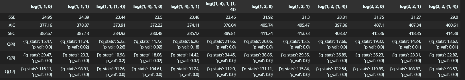
아래의 (p,d,q) tuple에 관해 test했다.
(1,1,0), (1,1,1), (1,1,[1,4]), (1,2,0), (1,2,1), (1,2,2), (2,2,0), (2,2,1), (2,2,2)
그 결과는 아래와 같다. Ljung Q-box test는 모델의 잔차가 white-noise process를 따르는지를 알려준다, p-value를 기반으로하였을 때 4, 8, 12까지의 잔차들간 상관성이 없음을 유의수준 95% 내에서 검정하였다.
추가적으로 Sum of Squared Errors (SSE), Akaike Information Criterion (AIC), Schwarz Bayesian Criterion (SBC)도 고려하여 모델을 판단하였을 때 (1,1,0), (1,1,1) 후보를 선택했다.

+) ARIMA(1,1,[1,4]) 또한 선택하는 것이 타당해보이나, lag 4의 residual을 추가하는 것이 overfitting으로 이어질 수 있다고 판단하였다(월별 데이터이기에 더욱 더).
log transformed data test
후보군은 다음과 같다. (1,1,0), (1,1,1), (1,1,[1,4]), ([1,4],1,0), ([1,4], 1, 1), ([1,4],1,[1,4]), (1,2,0), (1,2,1), (1,2,[1,4]), (2,2,0), (2,2,1), (2,2,[1,4])
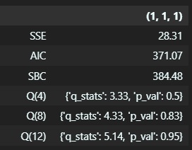
결과를 토대로 ARIMA(1,1,1)과 (1,1,0) 모델을 선택하였다.
아래의 그림은 log-transformed ARIMA(1,1,1)에 관한 잔차 분석을 시각화한 것으로 상관성이 없음을 눈으로 확인 가능하다.

Forcast
이후 선정된 4개의 모델에 관해 out-sample data을 이용하여 forcast 성능을 확인해보았다. 본 글에서 log-ARIMA는 log-transformed된 데이터를 사용한 ARIMA모델을 의미한다.
f1은 ARIMA(1,1,0), f2는 ARIMA(1,1,1), f3는 log-ARIMA(1,1,0), f4는 log-ARIMA(1,1,1)을 의미한다.
보면 4 모델 모두 시각적으로 보았을 때 잘 예측을 하고 있음을 확인 가능하며, 동시에 살짝 lagged된 형태로 예측을 하고 있음을 알 수 있다. 이는 모델 특성에서 기인된 것으로 보인다.

또한 잔차분석 결과 특정 pattern이 나타나지 않음을 확인 가능하다.

MAPE 결과는 다음과 같다.

SARIMA
Sesonal ARIMA 모델은 ARIMA에서 Seasnoal, 즉, 계절적 효과를 추가한 모델이다. 모델은 (p,d,q) * (P,D,Q,M)의 인자로 구성되며, 이 중 (p,d,q)의 경우 ARIMA와 비슷하며 (P,D,Q,M)의 경우 Seasoanl term을 담당하며 M이 그 반복되는 간격을 설정한다.
ACF와 PACF를 통해 M=4, 12로 설정하는 것이 합리적임을 그림을 통해 확인 가능했다. 또한 log-transformed한 경우가 보다 안정적임을 확인했기에 이에 관해서만 실험을 진행하였다.

위의 2가지 case에 관해 ADF와 KPSS를 확인한 결과는 아래와 같고, 두 경우 모두 정상성을 띔을 확인 가능하다.

다만, ACF와 PACF를 두 데이터에 관해 그려보았을 때, 좌측이 M=4인 경우 우측이 M=12인 경우인데 4인 경우에는 여전히 계절적 특성이 보임을 확인가능하다. SARIMA 모델에서 계절적차분을 통해 이러한 특성을 제거하려고하는것이 목적이기에 M=12를 선택하였다.

최종적으로 SARIMA(1,1,1)(1,1,1,12) 모델을 선택하였다.
Ljung-Q box statistic test를 진행한 결과는 아래와 같으며, 모델이 합리적임을 확인가능하다.
이후 Forcasting을 진행한 결과 또한 아래와 같다.
MAPE의 경우 2.4%로 매우 향상된 결과를 보였고, 시각적으로 확인된 결과에서도 이전과 다르게 lagged된 예측값을 제공하지 않으며, 잔차 또한 패턴이 없음을 확인할 수 있다.


Code Implement
추가적으로 자세한 코드는 아래의 github을 참고하면 된다!
https://github.com/zinhyeok/AirPassenger_TAF_ARIMA
GitHub - zinhyeok/AirPassenger_TAF_ARIMA: 2024-4-1 Time series analysis 수업 수강 과제, ARIMA 모델 및 unit root test
2024-4-1 Time series analysis 수업 수강 과제, ARIMA 모델 및 unit root test - zinhyeok/AirPassenger_TAF_ARIMA
github.com
'전공&대외활동 이야기 > 전공 프로젝트 모음' 카테고리의 다른 글
[Applied Data Analytics] Pickle? CSV? 데이터 파일의 형식에 관해 (0) 2024.03.31 [금융공학개론(INE3083)]Portfolio Management Project using Markowitz Model and Time series(Using RNN, LSTM, GRU) (2) 2023.11.08