[Time-series] Are Transformers Effective for Time Series Forecasting? (AAAI 2023, Ailing Zeng et al.)

https://arxiv.org/abs/2205.13504

Are Transformers Effective for Time Series Forecasting?

논문코드: https://github.com/cure-lab/LTSF-Linear

GitHub - cure-lab/LTSF-Linear: [AAAI-23 Oral] Official implementation of the paper "Are Transformers Effective for Time Series F

 

기존의 시계열(최근 Transfomer 기반 시계열 방법론들) 모델들과 다르게 Transfomer기반 모델이 아닌 MLP기반 모델을 이용한 방법론(비교군)을 제시하며, 기존의 transfomer 기반의 시계열 모델들의 성능이 과장된 것은 아닌지 의문을 제시한다. 이는 기존의 연구들이 대다수 효율적인 self-attention 방법론(logsparse, infomer 등)에 집중하고 있지만, Transfomer 방법론이 temporal relation을 잘 추출하지 않고 있으며,  LTSF task에 효과적이지 않음을 주장함. 

 

Fedfomer, Infomer 등의 모델(당시 SOTA)과 결과를 비교하고, 또 다양한 시각에서 모델의 성능을 확인한다. 

본 리뷰는 논문을 제외하고, 아래의 2 자료를 추가 참고하였다. 
[DSBA] Lab Seminar 2022: https://www.youtube.com/watch?v=J5Pl5a_mXfE
Hugging Face 블로그 글인 Yes, Transformers are Effective for time series Forecasting을 https://huggingface.co/blog/autoformer

BackGround

NLP, 즉 자연어처리를 함에 있어서 Transfomer base 모델들은 최근에도 꾸준히 좋은 모델을 보여주고 있으며, 이는 자연어 데이터 또한 마찬가지로 Sequencial한 data이기 때문이다. 

하지만 본 논문은 간단한 MLP Structuer만으로(특히 1-layer linear model 만을 이용하여 prediction을 수행) Time series forcasting을 진행한다. 

Time series Data

시계열 데이터는 시간에 따라 변하는 데이터로 구성되어 있으며, 이 값들은 서로 상관관계를 가진다. 

자세한 내용은 추가링크 참고

 

또한 예측에 있어서 2가지 방법을 적용가능하고, 이는 sequence data들의 예측에서도 동일하게 적용된다. 

Lim Bryan and Stefan Zohren, "Time series forcasting with deep learning: a servey"

Iterative Methods는 train data를 이용해서 다음 data를 순차적으로 예측하는 모델이다. 이때 예측한 결과값을 다음 예측에 동일하게 이용한다. 이런 경우 예측이 올바르지 않을 경우 뒤 부분의 예측이 모두 어긋나는 문제가 생기게 된다. 

 

Direct Method는 Predict의 여러 step에 해당하는 정보들을 동시에 예측하는 방법이다. 즉. ground truth한 input을 받는다. 

 

Transfomer based model의 문제점 

1. Computationally Expensive

 

2. Unable to capture global view

FEDformer: Frequency Enhanced Decomposed Transformer for Long-term Series Forecasting : https://arxiv.org/abs/2201.12740

 

그림에서 알수 있듯이 Transfomer알고리즘이 기존의 LSTM이나 RNN방법론보다 long term한 정보를 담을 수 있지만 그래도 여전히 Global한 데이터 특성을 담지 못함을 확인 가능하다. 

왼쪽 그림을 보면 알 수 있듯, 노란색 predict는 계속 상승할 것으로 예측하지만, 실제로는 그렇지는 않은 모습을 보여준다. 

오른쪽 그림은 frequency는 잘 예측한 반면, trend예측에 실패한 모습을 보여준다. 

 

아래에서부터는 본 논문에서 말하는 추가적인 한계점들이다. 

 

3. Multi head attention mechanism의 문제점(NLP 데이터와의 차이)

NLP의 Permutation invariant한 특성

Multi head attention이 사용된 NLP 분야에서는 긴 Sequence의 data에서 Semantic correlation을 추출하는 것이 주요했다. 

즉, 문장의 순서나 data가 다르더라도, 동일한 의미를 추출하는 것이 주요했기에, 순서가 바뀌어도 어느정도의 Sequence까지는 Permutaion invariant했다. 

그러나 Time series는 numerical data이고, Semantic한 정보가 부족하다. 

대표적인 time series 데이터 셋인 Finance dataset과 Energy Dataset을 보더라도 시계열에서 주요한 것은 각 element간의 상관관계보다는 Continuous한 set of point로 이루어져 있기에, 전체적인 변동의 추세, 즉, temporal dynamic을 포착하는 것이 중요하다. 

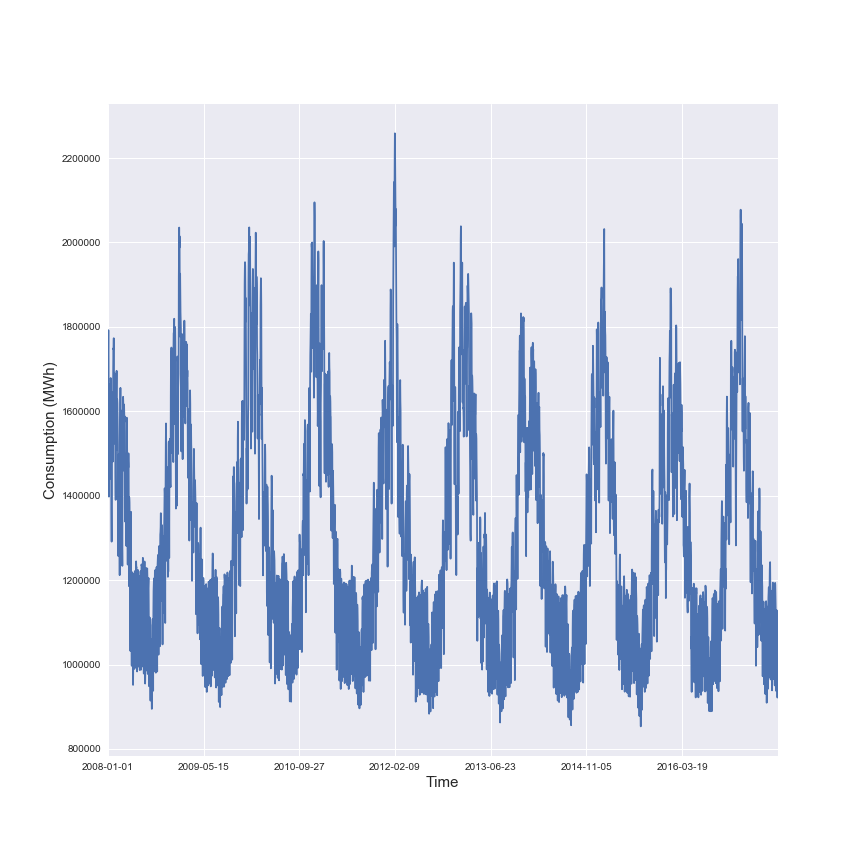
왼: 나스닥 주가, 오: French Electricity dataset

 

하지만 transomer에서는 long term sequence data에 관해 이런 temporal한 정보를 잘 추출하지 못한다. 

특히 positional encoding이나 temporal encoding을 통해 순서에 관한 정보를 넣어주려고 하지만, 이로 충분치 않다고 주장한다. 

또한 추가적으로 Autoregressive한 구조를 기반으로 함으로 Error Accumlation 문제가 발생한다. 

 

4. Positonal Encoding is really working?

기존 transfomer모델에서는 다양한 positional encoding을 사용하여 ordering information을 보존하려고 하지만, self-attention 매커니즘 상 positonal encoding정보의 손실을 피하는 것은 불가능하다. 

( However, self-attention is permutationinvariant and “anti-order” to some extent. While using various types of positional encoding techniques can preserve some ordering information, it is still inevitable to have temporal information loss after applying self-attention on top of them - 논문 intro 발췌)

 

본 논문에서는 매우 간단한 선형기반의(multi regression model) 모델을 제시함으로서 기존의 transfomer 모델들과 비교, 또한 다양한 상황(positonal check, long window 에서의 성능 비교)에서 모델의 성능을 확인한다. 

추가적으로 논문에서 기존의 transfomer와의 성능을 비교한 논문(Transformer 기반 LTSF 솔루션들은 기존 방법론들에 비해 개선된 예측 정확도를 보여주는 논문들)에서의 모델들은( Stock price prediction using the arima model, Adebiyi A Ariyo et al.IEEE,  Neural machine translation by jointly learning to align and translate by Dzmitry e al, 등 4편 제시)는 autro regressive model이라 multi-step 문제인 LTSF문제에 해당 결과를 제시하는 것은 맞지 않다고 

 

Transformer-Based LTSF Solutions(기존 transfomer 기반 모델 구조)

Fig1 in paper

 

우선 앞서, 기존의 transfomer based model을 LTSF에 적용할 때에는 두가지 한계점이 존재했다. 

1. original self attention의 quadratic time complexity/moemory complexity

2. autoregressive 한 decoder로 인한 error accumulation

이를 위해 현재의 transfomer based LTSF 모델들은 위의 구조를 가진다. 

[Time series decompositon]

 zero-mean normalization: data preporcessing 과정에서 흔히 사용하는 방법

Autofomer: seasonal-trend decompositon을 적용/ moving average kernel을 이용해 시계열 데이터의 trend-cyclical component를 추출

Fedfomer: 전문가 전략과 다양한 kernel size의 moving avergage 적용

[Input embedding strategies]

시계열의 time series적인 특성, 즉 position을 보존하는 문제는 매우 주요하다.

하지만, transfomer 기반 모댈의 selkf-attention layer는 이를 보존하지 못하기 때문에  SOTA Transformer 기반 모델들은 여러 embedding을 input sequence에 활용하며 애래의 예시가 있다. 
+ fixed positional encoding channel projection embedding learnable temporal embeddings
+ temporal convolution layer( Enhancing the Locality and Breaking the Memory Bottleneck of Transformer on Time Series Forecasting (NeurIPS 2019))를 통한 temporal embeddings or  using learnable timestamps(AutoFomer)를 통한 embedding

[Self-attention schemes]

Transfomer에서 기존에 사용되던 self-attention mechanism은 L^2의 시간복잡도를 가지기에 이를 줄이기 위한 전략을 제시 

1. LogTrans와 Pyraformer는 self-attention 메커니즘에 sparsity bias 를 도입

• LogTrans는 Logsparse mask 를 사용하여 computational complexity를 O(LlogL)로 감소
• Pyraformer는 hierarchically multi-scale temporal dependencies 를 포착하는 pyramidal attention 을 통해 time/memory complexity를 O(L)로 감소

2. Infomer& Fedformer는 self-atttention matrix에 low-rank porperty 사용

• Informer는 ProbSparse self-attention 메커니즘과 self-attention distilling operation 을 통해 complexity를 O(LlogL)로 감소
• FEDformer는 random selection으로 Fourier enhanced block 과 wavelet enhanced block 을 설계해 complexity를 O(L)로 감소
• Autoformer는 original self-attention layer를 대체하는 series-wise auto-correlation 설계\

[Decoders]

위에서 언급했듯. auto regressive한 방법으로 output을 생성하기에 느린 추론 속도와 error accumulaiton발생 이를 해결하기 위해 아래의 방법론들이 제시 

• Informer는 DMS forecasting을 위한 generative-style decoder 를 설계
• Pyraformer는 fully-connected layer를 Spatio-temporal axes와 concatenating하여 decoder로 사용
• Autoformer는 최종 예측을 위해 trend-cyclical components와 seasonal components의 stacked auto-correlation 메커니즘을 통해 재정의된 decomposed features를 합침
• FEDformer는 최종 결과를 decode하기 위해 frequency attention block을 통한 decomposition scheme를 사용]

즉, Transfomer 모델은 pair wised element간 semantic corrlation을 모델링하는 것이나, numerical 한 data의 경우 데이터 간 point-wise corrlation보다는 연속적인 데이터 집합에서의 temporal relation을 뽑아내는 것이다. 그렇기에 데이터의 positional encdoing부분이 무엇보다 주요하다. 

 

LTSF-linear 모델(An embarassingly simple baseline)

LTSF 모델의 기본적인 수식은 weighted sum만으로 미래 예측을 하는것, 즉, 과거 시계열 데이터를 회귀식으로 이용하는 것이다. 결국 가중합으로 표현하는 것이다.

import torch
import torch.nn as nn
import torch.nn.functional as F
import numpy as np

class Model(nn.Module):
    """
    Just one Linear layer
    """
    def __init__(self, configs):
        super(Model, self).__init__()
        self.seq_len = configs.seq_len
        self.pred_len = configs.pred_len
        
        # Use this line if you want to visualize the weights
        # self.Linear.weight = nn.Parameter((1/self.seq_len)*torch.ones([self.pred_len,self.seq_len]))
        self.channels = configs.enc_in
        self.individual = configs.individual
        if self.individual:
            self.Linear = nn.ModuleList()
            for i in range(self.channels):
                self.Linear.append(nn.Linear(self.seq_len,self.pred_len))
        else:
            self.Linear = nn.Linear(self.seq_len, self.pred_len)

    def forward(self, x):
        # x: [Batch, Input length, Channel]
        if self.individual:
            output = torch.zeros([x.size(0),self.pred_len,x.size(2)],dtype=x.dtype).to(x.device)
            for i in range(self.channels):
                output[:,:,i] = self.Linear[i](x[:,:,i])
            x = output
        else:
            x = self.Linear(x.permute(0,2,1)).permute(0,2,1)
        return x # [Batch, Output length, Channel]

예를 들어 72 window size, 100예측일때 172일 전의 data 중 72개를 가지고 100개 예측(winodw내에서)하는 선형 식 만들어 해당 가중치를 그대로 현재 시점으로부터 과거의 72개의 data를 가지고 미래의 100개를 예측하는 수식에 쓴다. 

 

또한 이를 조금 더 발전시켜서 Nlinear와 Dlinear모델을 제시하는데, 

Nlinear의 경우 가장 마지막 값을 빼서 모델을 학습시키고 이후 predict 직전 다시 그 값을 더해서 실제 값이 존재하는 분포로 이동하여 Distribution shift 문제를 방지하고자 하는 방법론이다(이후 최종 prediction 전에 더해줌)

Distribution shift
데이터가 상승하거나 하락하는 추세를 지닐 경우 학습데이터의 평균과 분산으로 데이터를 단순히 정규화 시키면 평가 데이터에 분포가 이동하여 예측성능이 크게 하락하는 것을 의미 

distiribution shift of data

def forward(self, x):
    # x: [Batch, Input length, Channel]
    seq_last = x[:,-1:,:].detach()
    x = x - seq_last
    if self.individual:
        output = torch.zeros([x.size(0),self.pred_len,x.size(2)],dtype=x.dtype).to(x.device)
        for i in range(self.channels):
            output[:,:,i] = self.Linear[i](x[:,:,i])
        x = output
    else:
        x = self.Linear(x.permute(0,2,1)).permute(0,2,1)
    x = x + seq_last
    return x # [Batch, Output length, Channel]

 

Dlinear의 경우 Decompostion 방법(AutoFomer와 Fedfomer에서 사용)을 이용, trend-cyclical data와 remainder data로 분해한 decomposed된 data에 관해 Linear한 방법으로 각각 예측한 뒤 합하는 방법이다. 

이때 분해에 있어서 이동평균값을 Trend라고 보고 이를 제거한 데이터와 해당하는 값으로 분리한다. 

(실제 코드 확인 시 25 time stamp의 고정된 moving avergae를 이용하는 것을 확인 가능하다)

DLinear은 시계열 데이터의 명확한 추세와 주기성이 있을 때 더 좋은 성능을 가질 것으로 예측된다. 

춫

class series_decomp(nn.Module):
    """
    Series decomposition block
    """
    def __init__(self, kernel_size):
        super(series_decomp, self).__init__()
        self.moving_avg = moving_avg(kernel_size, stride=1)

    def forward(self, x):
        moving_mean = self.moving_avg(x)
        res = x - moving_mean
        return res, moving_mean

Experiment 

Dataset

dataset은 아래와 같으며, 보통 LTSF에서 많이 사용되는 benchmark dataset이다

 

Evalutaion metric으로는 MSE와 MAE를 사용하였다. 

Comparison with Transomer *(main result)

table 2 from paper(for mutlivariate model)

비교한 모델은 5개의 Transfomer 기반 방법론인 FEDformer, Autoformer, Informer, Pyraformer, LogTrans과 

3개의 제시모델, 그리고 Repeat은 단순히 look-back window의 마지막 값만 반복하는 base모델이다. 

 

결과를 보면 LTSF-linear의 성능이 SOTA인 FEDFomer보다 대부분 20~50%까지 높은 성능을 보인다. 이는 변수간 correlation을 고려하지 않았음에도 놀라운 성능을 보여준다

Nlinear와 Dlinear는 Distribution shift와 trend-seasonality를 다루는 능력이 우세함을 확인가능하다. 

또한 단순 Repeat model의 경우에도 long-term seasonal data (e.g., Electricity and Traffic)에서는 좋지 않은 성능을 보여주지만, Exchange rate에서는 놀라울 정도로 좋은 성능을 보여준다(transfomer 대비 45%). 이는 명확한 추세성이 없는 경우 noise에 transfomer model들이 overfitting이 된것이 아닌지에 관해 의문을 제시한다. 

 

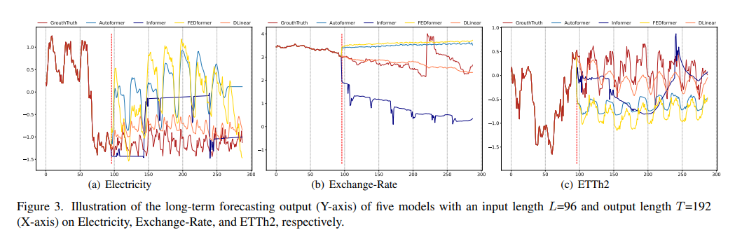
Ground-truth와 비교한 그림을 보면 알 수 잇듯이( Electricity(Sequence 1951, Variate 36), Exchange-Rate(Sequence 676, Variate 3), ETTh2(Sequence 1241, Variate 2), input length L=96 and output length T=192 ) transfomer model이 각기 다른 temoporal pattern을 보이는 데이터셋들 중 exchnage rate를 잘 예측하지 못하는 것을 확인 가능. 

Electricity에서는 scale예측에, ETTh애서는 bias를 잘 못 예측하는 것을 확인 가능하다. 

 

아래는 appendix에 포함된 자료로 univariate model로써도 잘 작동한다는 것을 보여준다

 

이후 나온 결과들은 Transfomer가 LTSF에 적합하지 않은 이유를 하나씩 제기하며 결과로 보여준다. 

Can existing LTSF-Transformers extract temporal relations well from longer input sequences?

lookback window size는 얼마나 많은 과거 data를 참조하는지를 정해주는 크기에, 예측 정확도에 많은 영향을 끼친다. 

그리고 일반적으로 temporal relation 추출을 잘한 모델이라면, 큰 look-back window size를 통해 더 좋은 결과를 보여주어야한다. 

하지만

👎 Transformer 기반 모델들의 성능은 기존 연구의 결과와 동일하게 look-back window size가 커지면서 성능이 악화되거나 안정적으로 유지(96 정도가 적합함) 이는 더 긴 시퀀스가 주어질 경우 노이즈에 과적합되는 경향이 있음을 보임
👍 반면 LTSF-Linear 모델은 look-back windows sizes가 커짐에 따라 성능이 향상

What can be learned for long-term forecasting?

 

단기 예측과 달리 장기예측은 모델의 추세와 주기를 정확하게 포착하는 것이 주요하기에 look-back window내의 동적인 변화가 덜 주요하다. 

즉, 예측 시간이 멀어질 수록 look-back window 자체의(크기가 아니라 어떤 data를 참조하느냐)의 영향을 줄어들어야한다. 

이 가설을 검증하기 위해 (i). 원래 입력인 L=96 설정 (Close로 불림)과 (ii). 원래 96개의 시간 단계 이전인 L=96 설정 (Far로 불림)을 비교한다. 

그 결과 Transfomer 모델의 성능의 약간의 감소를 확인 가능한데, 이는 데이터 셋에서 인접한 시계열 순서에서만 포착하는 것이 아닌지 의문을 준다. 또한 이는 적은 수의 매개변수만으로도 주기성 등 정보를 포착하는데 충분하다는 것을 보여주며 Transfomer의 과적합 문제를 제기한다. 

 

Can existing LTSF-Transformers preserve temporal order well?

 

표 5에서는 학습 전에 원시 입력을 섞어봅니다. 두 가지 data 변형(shuffle)전략을 사용합니다: Shuf.는 전체 입력 시퀀스를 무작위로 섞고, Half-Ex.는 입력 시퀀스의 첫 번째 절반과 두 번째 절반을 교환한다.

즉. 이를 통해서 순서에 얼마나 영향을 받는지를 확인 가능한데

그 결과 Transomer 방법론에서는 성능하락이 일어나지 않는 것을 확인 가능하고, 이는 시계열에서도 permutaion invariant한 특징이 적용되여 temporal order가 잘 반영되지 않음을 보여준다

 

How effective are different embedding strategies?

Embedding 방법론들 중 어떤 것이 유의한지를 확인한 표이다.

 

 Informer

•  positional embeddings가 없을 경우 예측 오류가 크게 증가
• timestamp embeddings가 없는 경우에는 예측 길이가 길어짐에 따라 성능이 점차 하락
  (Informer가 각 토큰에 대해 단일 time step을 사용하기 때문에 temporal information을 토큰에 도입해야 함)

FEDformer와 Autoformer는 각 토큰마다 단일 time step을 사용하지 않고 temporal information을 도입하기 위해 timestamps의 시퀀스를 입력

• 고정된 positional embeddings 없이도 비슷하거나 더 나은 성능을 달성
• global temporal information loss 때문에 timestamp embeddings이 없으면 Autoformer의 성능은 빠르게 하락
• FEDformer는 temporal inductive bias를 도입하기 위한 frequency-enhanced module 덕분에 position/timestamp embeddings을 제거해도 성능이 덜 하락

 

Code Implementation

code implementation은 공식 논문 github과(위의 링크 참조). https://today-1.tistory.com/60 를 참조하여 작성하였다 

✔ Is linear Nlinear Dlinear different?

미팅 중 교수님께서 주신 의문, linear 모델이기 때문에 data를 이리저리 substracting하는 것이 의미가 있느냐?라는 질문이었다. 이를 code를 통해 명확히 더 확인 가능했다. 

 

https://colab.research.google.com/drive/1NKu0XmIwIzyYJ5mfsb7iZLqo7oIfilGb?usp=sharing

LTSF-linear.ipynb

Model 코드

각 model code는 공식 github을 바탕으로 작성하되, config부분은 직접 값을 대입할 수 있게 변경하였다. 

class LTSF_Linear(torch.nn.Module):
    def __init__(self, window_size, forcast_size, individual, feature_size):
        super(LTSF_Linear, self).__init__()
        self.window_size = window_size
        self.forcast_size = forcast_size
        self.individual = individual
        self.channels = feature_size
        if self.individual:
            self.Linear = torch.nn.ModuleList()
            for i in range(self.channels):
                self.Linear.append(torch.nn.Linear(self.window_size, self.forcast_size))
        else:
            self.Linear = torch.nn.Linear(self.window_size, self.forcast_size)

    def forward(self, x):
        if self.individual:
            output = torch.zeros([x.size(0), self.forcast_size, x.size(2)],dtype=x.dtype).to(x.device)
            for i in range(self.channels):
                output[:,:,i] = self.Linear[i](x[:,:,i])
            x = output
        else:
            x = self.Linear(x.permute(0,2,1)).permute(0,2,1)
        return x

class LTSF_NLinear(torch.nn.Module):
    def __init__(self, window_size, forcast_size, individual, feature_size):
        super(LTSF_NLinear, self).__init__()
        self.window_size = window_size
        self.forcast_size = forcast_size
        self.individual = individual
        self.channels = feature_size
        if self.individual:
            self.Linear = torch.nn.ModuleList()
            for i in range(self.channels):
                self.Linear.append(torch.nn.Linear(self.window_size, self.forcast_size))
        else:
            self.Linear = torch.nn.Linear(self.window_size, self.forcast_size)

    def forward(self, x):
        seq_last = x[:,-1:,:].detach()
        x = x - seq_last
        if self.individual:
            output = torch.zeros([x.size(0), self.forcast_size, x.size(2)],dtype=x.dtype).to(x.device)
            for i in range(self.channels):
                output[:,:,i] = self.Linear[i](x[:,:,i])
            x = output
        else:
            x = self.Linear(x.permute(0,2,1)).permute(0,2,1)
        x = x + seq_last
        return x

class moving_avg(torch.nn.Module):
    def __init__(self, kernel_size, stride):
        super(moving_avg, self).__init__()
        self.kernel_size = kernel_size
        self.avg = torch.nn.AvgPool1d(kernel_size=kernel_size, stride=stride, padding=0)

    def forward(self, x):
        front = x[:, 0:1, :].repeat(1, (self.kernel_size - 1) // 2, 1)
        end = x[:, -1:, :].repeat(1, (self.kernel_size - 1) // 2, 1)
        x = torch.cat([front, x, end], dim=1)
        x = self.avg(x.permute(0, 2, 1))
        x = x.permute(0, 2, 1)
        return x

class series_decomp(torch.nn.Module):
    def __init__(self, kernel_size):
        super(series_decomp, self).__init__()
        self.moving_avg = moving_avg(kernel_size, stride=1)

    def forward(self, x):
        moving_mean = self.moving_avg(x)
        residual = x - moving_mean
        return moving_mean, residual

class LTSF_DLinear(torch.nn.Module):
    def __init__(self, window_size, forcast_size, individual, feature_size, kernel_size=25):
        super(LTSF_DLinear, self).__init__()
        self.window_size = window_size
        self.forcast_size = forcast_size
        self.decompsition = series_decomp(kernel_size)
        self.individual = individual
        self.channels = feature_size
        if self.individual:
            self.Linear_Seasonal = torch.nn.ModuleList()
            self.Linear_Trend = torch.nn.ModuleList()
            for i in range(self.channels):
                self.Linear_Trend.append(torch.nn.Linear(self.window_size, self.forcast_size))
                self.Linear_Trend[i].weight = torch.nn.Parameter((1/self.window_size)*torch.ones([self.forcast_size, self.window_size]))
                self.Linear_Seasonal.append(torch.nn.Linear(self.window_size, self.forcast_size))
                self.Linear_Seasonal[i].weight = torch.nn.Parameter((1/self.window_size)*torch.ones([self.forcast_size, self.window_size]))
        else:
            self.Linear_Trend = torch.nn.Linear(self.window_size, self.forcast_size)
            self.Linear_Trend.weight = torch.nn.Parameter((1/self.window_size)*torch.ones([self.forcast_size, self.window_size]))
            self.Linear_Seasonal = torch.nn.Linear(self.window_size,  self.forcast_size)
            self.Linear_Seasonal.weight = torch.nn.Parameter((1/self.window_size)*torch.ones([self.forcast_size, self.window_size]))

    def forward(self, x):
        trend_init, seasonal_init = self.decompsition(x)
        trend_init, seasonal_init = trend_init.permute(0,2,1), seasonal_init.permute(0,2,1)
        if self.individual:
            trend_output = torch.zeros([trend_init.size(0), trend_init.size(1), self.forcast_size], dtype=trend_init.dtype).to(trend_init.device)
            seasonal_output = torch.zeros([seasonal_init.size(0), seasonal_init.size(1), self.forcast_size], dtype=seasonal_init.dtype).to(seasonal_init.device)
            for idx in range(self.channels):
                trend_output[:, idx, :] = self.Linear_Trend[idx](trend_init[:, idx, :])
                seasonal_output[:, idx, :] = self.Linear_Seasonal[idx](seasonal_init[:, idx, :])
        else:
            trend_output = self.Linear_Trend(trend_init)
            seasonal_output = self.Linear_Seasonal(seasonal_init)
        x = seasonal_output + trend_output
        return x.permute(0,2,1)

학습 및 Test

hyperparameter는 아래와 같이 설정하였다. 즉, 96 window size(History of L)에서 forcast를 96(Future T timesteps)개를 하였다(추가로  논문의 run_longExp.py 파일 참조)

이는 논문에서 언급한 Input 숫자를 따른 것이다(FedFomer와 동일한 setting을 했다고 밝혔고, 아래는 Fedfomer의 실험 설계 내용)

 

Multivariate long-term series forecasting results on six datasets with input length I = 96 and prediction length O ∈ {96, 192, 336, 720} (For ILI dataset, we use input length I = 36 and prediction length O ∈ {24, 36, 48, 60})

 

epoch_size = 10
lr = 0.0001
batch_size = 32
#early stop 조건
patience =5
window_size = 96
forcast_size= 192

 

학습 코드의 일부는 아래과 같다. 

model_name = 'LTSF_Linear'

model =  LTSF_Linear(
                      window_size=window_size,
                      forcast_size=forcast_size,
                      individual=False,
                      feature_size=1,
                      )

model.to(device)
criterion = nn.MSELoss()
optimizer = optim.Adam(model.parameters(), lr=lr)

train_loader = DataLoader(train_ds, batch_size=batch_size, shuffle=True)
valid_loader = DataLoader(valid_ds, batch_size = batch_size, shuffle=False)
test_loader = DataLoader(test_ds, batch_size=batch_size, shuffle=False)


train_loss_list = []
valid_loss_list = []
test_loss_list = []



if __name__ == '__main__':
    best_val_loss = float('inf')
    since = time.time()
    print(f'Training  Model on {device}\n{"=" * 44}')
    for epoch in range(1, epoch_size+1):
        epoch_start = time.time()
        train_loss = train(epoch)
        train_loss_list.append(train_loss)
        m, s = divmod(time.time() - epoch_start, 60)
        print(f'Training time: {m:.0f}m {s:.0f}s')

        val_loss = valid()
        valid_loss_list.append(val_loss)
        # Early stopping 체크
        if val_loss < best_val_loss:
            best_val_loss = val_loss
            early_stop_counter = 0
            torch.save(model.state_dict(), f'best_{model_name}_model.pth')  # 현재 가장 좋은 모델 저장
        else:
            early_stop_counter += 1
            if early_stop_counter >= patience:
                print("Early stopping!")
                break

    test_start = time.time()
    model.load_state_dict(torch.load(f'best_{model_name}_model.pth'))  # 가장 좋은 모델로 복원
    test_loss = test(model)
    m, s = divmod(time.time() - test_start, 60)
    print(f'Testing time: {m:.0f}m {s:.0f}s')

    m, s = divmod(time.time() - since, 60)
    print(f'Total Time: {m:.0f}m {s:.0f}s\nModel was trained on {device}!')

    result_list.append({"model": model_name,"Train": train_loss, "val": val_loss, "test": test_loss})
    predict_Linear = predict_result(model)
    # 각 텐서를 numpy 배열로 변환하여 리스트에 저장
    array_list = [tensor.detach().numpy() for tensor in predict_Linear]
    # 리스트 안의 모든 배열을 하나의 배열로 결합
    predict_Linear = np.stack(array_list)

결과

MSE 결과는 다음과 같다. 보면, MAE가 매우 크긴 하지만 DLinear > NLinear > Linear 가 성능이 좋음을 확인 가능하다. 

(다만 MSE가 논문의 결과보다 더 작게 나와서 코드를 다시 확인하고 있다)

직접 코드로 얻은 결과 Etth1에 관해 96 192결과

논문의 실험결과

Groundtruth와의 시각화 된 결과비교는 아래와 같다

Dlinear의 가중치를 시각화한 결과는 아래와 같다. 

실제로 Seasonal을 보면 주기적으로 가중을 주고 있는 것을 확인 가능하다.